Fully Connected Layers

This is part of a series on ML for generalists, you can find the start here.

Fully connected layers are the oldest part of our network. They're made up of perceptrons, the simplest possible neural network unit. They were invented in 1957 by Frank Rosenblatt.

A perceptron takes a list of input numbers, multiplies each by a weight, sums them up, and outputs a single number.

You have 3 inputs: [2, 5, 1]

The perceptron has 3 weights (one for each input), say: [0.4, -0.2, 0.6]

It also has a bias but we'll get to that shortly.

Here's how a perceptron calculates its output:

1. Multiply each input by its corresponding weight: [2, 5, 1] x [0.4, -0.2, 0.6]
   • 2 x 0.4 = 0.8
   • 5 x -0.2 = -1.0
   • 1 x 0.6 = 0.6
2. Add those together: 0.8 + -1.0 + 0.6 = 0.4 (+ bias)

Each perceptron has a single bias that gets added to its output. It lets us shift the output value up or down independent of the inputs. Why is that useful?

Let's say we're building a model to predict house prices based on their square metre size.

Without bias, our formula is: price = m² x weight

If our weight is 200, then a 1m² house costs €200, a 1000m² house costs €200,000 and a 0m² house costs €0.

But it's likely there's some minimum price to houses, even ruined cottages and empty plots. Without a bias we can't model that, it just doesn't fit.

If we add a bias to our formula: price = (m² x weight) + bias

We can keep our weight of 200 and set our bias as 50,000. Now a 1m² house costs €50,200, a 1000m² house costs €250,000 and a 0m² house costs €50,000.

In practice, we don't set a bias value ourselves, it's just another parameter of our model set by the training process.

Here's the full walk through of the operations inside a perceptron.

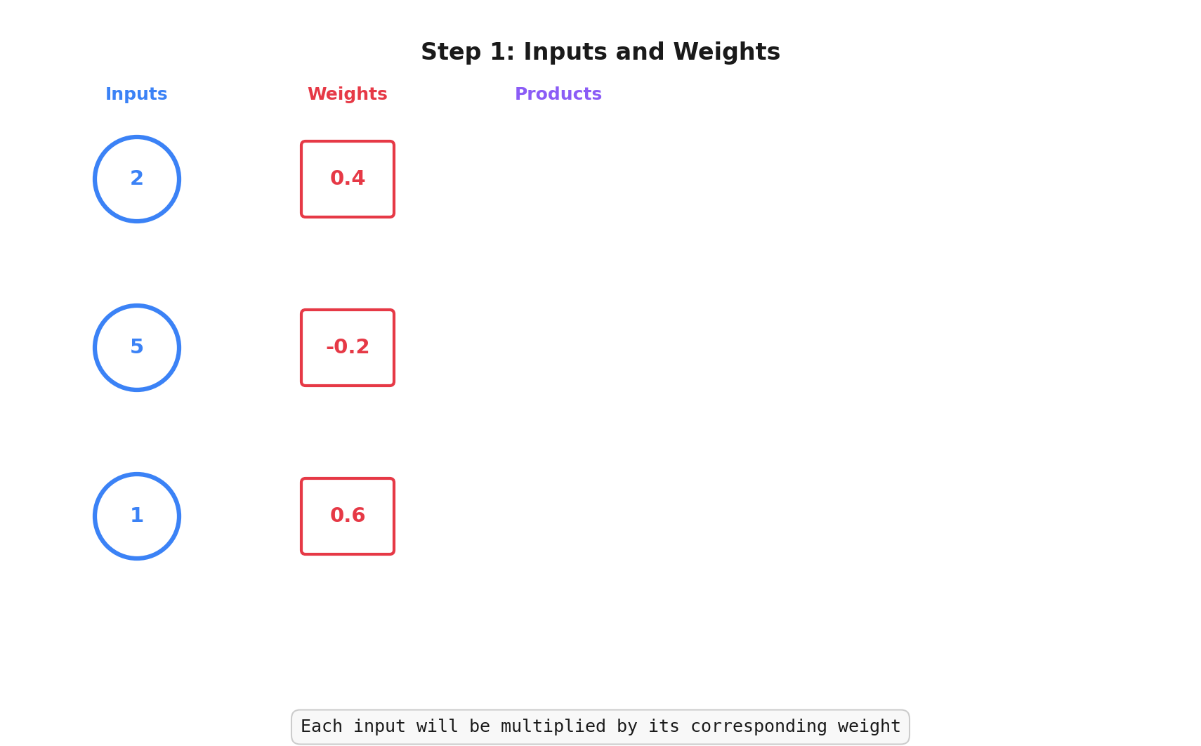
Step 1: We start with inputs and a weight for each of those inputs:

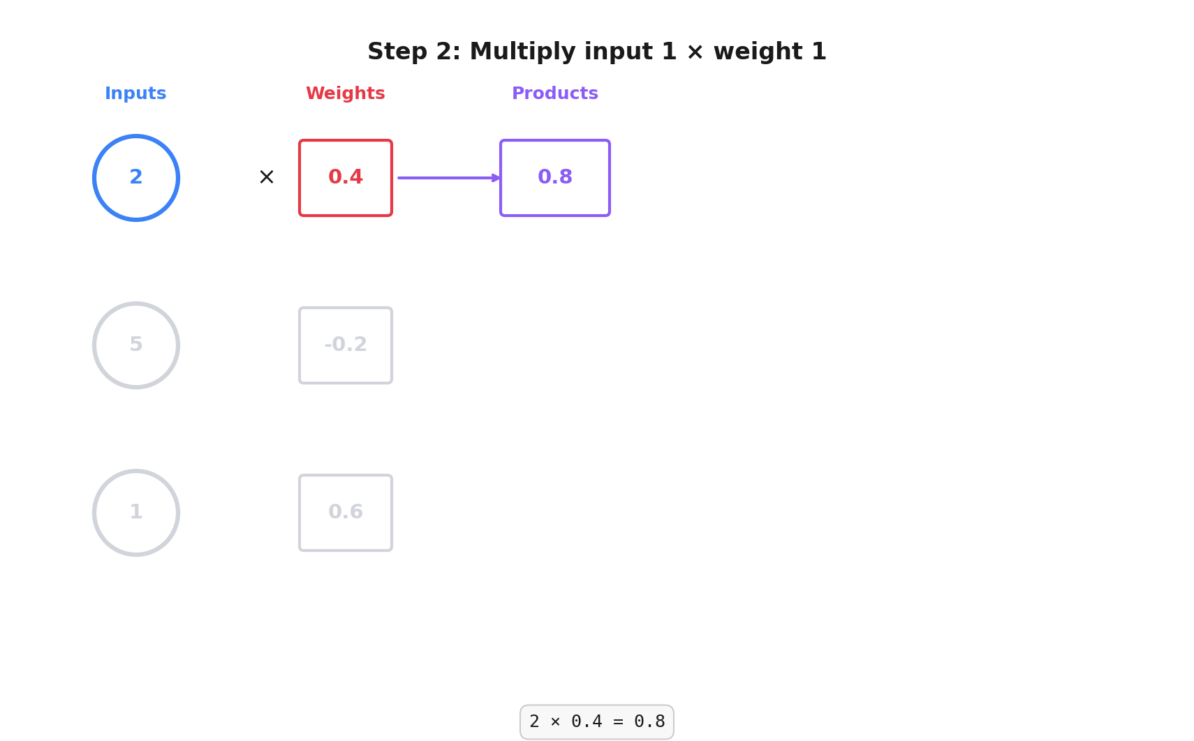
Step 2: We multiply the input values by their corresponding weights:

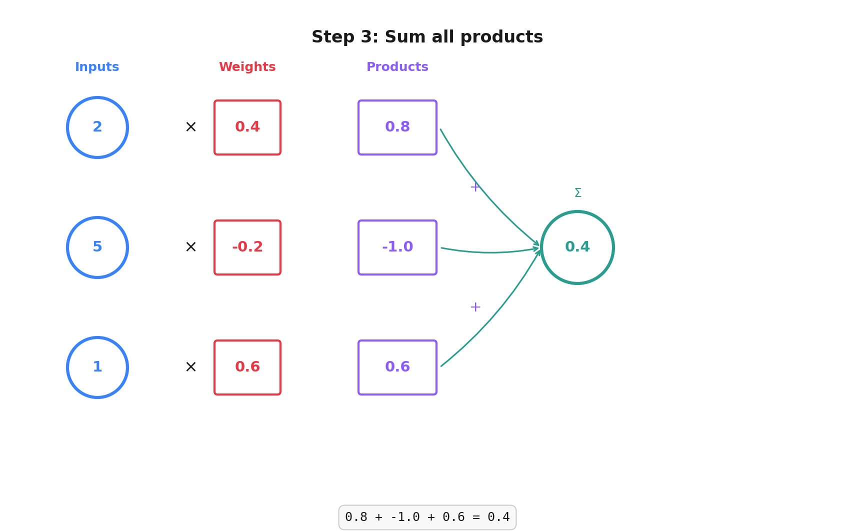
Step 3: We add their products together:

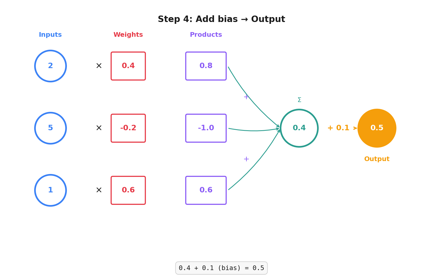
Step 4: We add our bias (0.1 in this example) and we get our output:

Here's the animated version:

Yes. They have a bias per output channel.

We can turn it off by setting nn.Conv2d(..., bias=False), but I'm going to skip why you might want to do that for now.

Here're the fully connected layers from our model:

nn.LazyLinear(out_features=64),
nn.Linear(in_features=64, out_features=2),

Why are they called nn.Linear? Maths! The operation is linear in a mathematical sense: output = input x weights + bias. In maths-speak, something is linear when scaling the input scales the output by the same amount.

What's the nn.LazyLinear? It lets us skip specifying the in_features parameter, PyTorch figures out the number of features when the layer is called for the first time.

We could calculate it ourselves from the output of the previous layer in our model. This lets us tweak things quickly without having to recalculate it ourselves.

Every input connects to every output in a fully connected layer. You'll often see it abbreviated as fc in PyTorch code.

nn.Linear(in_features=64, out_features=2),

We have 64 inputs and 2 outputs in this layer. That's 2 perceptrons with each perceptron having 64 inputs (and 64 weights), so this layer of the network will have 2 outputs (1 for each perceptron).

• nn.LazyLinear(out_features=64) takes those ~29 million and outputs just 64 values
• nn.Linear(in_features=64, out_features=2) reduces those 64 inputs to just 2 values -- our sine and cosine values

How does this layer know these are the sine and cosine values? It doesn't! We haven't trained it yet, we've only designed the shape of our model. We're going to push some images in at the top and we want two numbers out at the end. Once we train our model, those numbers will correspond to the angle of rotation of our input image. Magic!

In this post and the last, I've shown you snippets from our model. I've conveniently ignored some important lines.

class OrientationModel(nn.Module):
    def __init__(self):
        super().__init__()
        self.conv = nn.Sequential(
            nn.Conv2d(in_channels=1, out_channels=32, kernel_size=3, padding=1),
            nn.ReLU(),
            nn.MaxPool2d(kernel_size=2, stride=2),

            nn.Conv2d(in_channels=32, out_channels=64, kernel_size=3, padding=1),
            nn.ReLU(),
            nn.MaxPool2d(kernel_size=2, stride=2),

            nn.Conv2d(in_channels=64, out_channels=128, kernel_size=3, padding=1),
            nn.ReLU(),
            nn.MaxPool2d(kernel_size=2, stride=2),

            nn.Conv2d(in_channels=128, out_channels=128, kernel_size=3, padding=1),
            nn.ReLU(),
            nn.MaxPool2d(kernel_size=2, stride=2),

            nn.Conv2d(in_channels=128, out_channels=128, kernel_size=3, padding=1),
            nn.ReLU(),
            nn.MaxPool2d(kernel_size=2, stride=2),
        )

        self.flatten = nn.Flatten()
        
        self.fc = nn.Sequential(
            nn.LazyLinear(out_features=64),
            nn.ReLU(),
            nn.Linear(in_features=64, out_features=2),
        )

    def forward(self, x: torch.Tensor) -> torch.Tensor:
        x = self.conv(x)
        x = self.flatten(x)
        x = self.fc(x)
        return x

Luckily two of these are quick:

nn.Sequential lets you tell PyTorch what sequence of steps to take. It's a bit more functional programming style, you could equally apply all the layers in turn inside forward()

nn.Flatten takes the 3-dimensional tensor from our convolution layers and flattens it into a 1-dimensional tensor for the fully connected layers. They expect a flat list, this does the flattening.

In reality, the full input to that flatten call is a 4-dimensional tensor (batch, channels, height, width) and the output is a 2-dimensional tensor (batch, features), but I'll cover batches after we've trained our model.

For our problem, it doesn't matter if a feature appears a pixel to the left or a pixel lower in our image. We want some "translation invariance" -- we really only care about the significant features.

nn.MaxPool2d(kernel_size=2, stride=2) slides a 2x2 window (kernel_size) across each out_channel of our convolution layer, stepping by 2 (stride) each time and outputs only the largest value in each window.

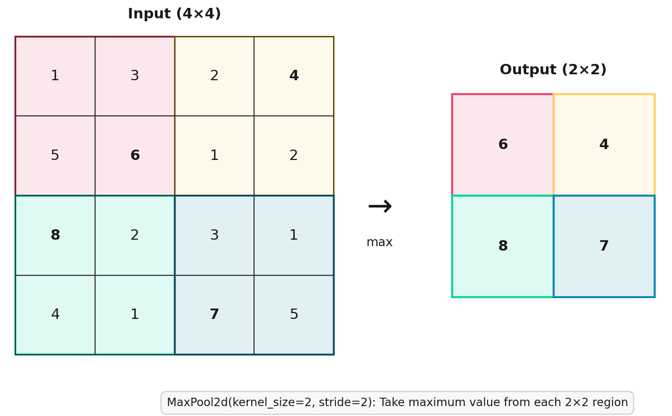
The top-left 2x2 block is [1, 3, 5, 6] for a max of 6. Top right is [2, 4, 1, 2] for a max of 4, and so on.

We keep the same number of output channels from the convolution layer, they're just smaller.

Our starting images are 480x480, we use MaxPool2d to halve 5 times: 240 → 120 → 60 → 30 → 15, for a 15×15 grid from each channel, or 225 values per channel. With 128 channels 128 x 225 that's 28,800.

Do we need to reduce this many times? Let's train and see.

This isn't a "learning" layer of the model, it isn't changed by training. It always performs the same operation. MaxPool2d reduces the amount of computation we need to do and helps our model to generalise a little more.

We're so close to training this model. Last concept is ReLU.